OCT Retinal-Layer Segmentation

Overview

I’m an optometrist. Most of my training has been in reading OCT scans, not writing the code that could eventually help interpret them. This project was my attempt to close that gap: to actually build, from raw pixels to trained model, a pipeline that turns an OCT B-scan into a quantitative, per-layer segmentation.

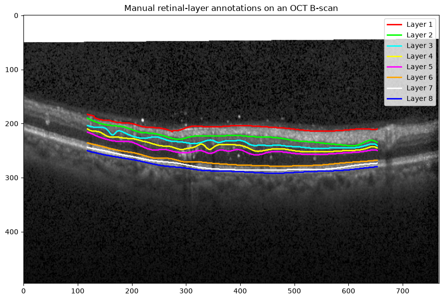
Optical coherence tomography gives you a cross-sectional view of the retina that’s genuinely beautiful to look at clinically, but turning that image into numbers (layer thicknesses, boundary positions, anything you could track over time or compare across patients) depends entirely on being able to identify the retinal boundaries reliably. Clinically, that’s often done manually or semi-automatically. I wanted to know whether I could build a model that did it end to end.

The dataset problem before the modeling problem

I used the Duke/Chiu 2015 OCT dataset: 10 subjects, 61 B-scans each, distributed as MATLAB .mat files with manual boundary annotations from two graders. Before any modeling happened, most of the real work was in getting from “raw MATLAB structs” to something a neural network could learn from.

Only a fraction of scans per subject actually had manual layer annotations. The preprocessing pipeline identified 110 annotated B-scans in total. Everything downstream depended on getting that filtering right, and on converting eight annotated boundary curves into clean, contiguous eight-region pixel-wise masks. That mask generation step needed real defensive care: a handful of boundary coordinates were malformed in ways that could silently produce negative NumPy indices and corrupt a mask without ever throwing an error. I validated mask generation across every annotated scan rather than trusting it would just work.

The other non-negotiable was subject-level splitting. It would have been easy to split by B-scan and get artificially good validation numbers, since scans from the same eye are highly correlated. I split by subject instead, so no eye appeared in both training and validation: a less flattering number, but a real one.

Building the model

With a working OCTLayerDataset (normalizing images to [0,1], returning integer class-label masks compatible with CrossEntropyLoss, retaining subject/scan provenance for debugging), I implemented a U-Net from scratch in PyTorch, with no pretrained backbone and no off-the-shelf segmentation library. Input is a single-channel 496×768 B-scan; output is an 8-channel map corresponding to background plus seven inter-boundary retinal layer regions.

Training used Adam optimization and Cross-Entropy loss over 20 epochs. I deliberately kept the pipeline modular: separate modules for .mat loading, mask generation, dataset construction, the model itself, and training/evaluation, so any one stage (loss function, architecture, dataset) could be swapped without touching the rest.

Results

The final Cross-Entropy U-Net reached:

• Mean Dice: 0.8328
• Mean IoU: 0.7233
• Pixel Accuracy: 0.9711

Layer	Dice
0	0.9899
1	0.8001
2	0.8870
3	0.7587
4	0.7282
5	0.8603
6	0.8299
7	0.8085

Layer 0 (background) was essentially solved. Layers 3 and 4 (thinner, more variable middle retinal layers) were consistently the hardest, which matches what I’d expect clinically: those are also the boundaries that are hardest to place precisely by eye.

What I got wrong on the first attempt

My instinct going in was that a combined Dice + Cross-Entropy loss would obviously do better. Dice loss directly optimizes the overlap metric I actually cared about, so why not target it directly?

I ran the controlled comparison anyway rather than assuming:

Model	Mean Dice	Mean IoU	Pixel Accuracy
U-Net + Cross-Entropy	0.8328	0.7233	0.9711
U-Net + Dice + Cross-Entropy	0.8282	0.7188	0.9720

The combined loss came out very slightly worse on the two metrics I actually cared about most, despite a marginal pixel-accuracy edge. So I kept the simpler Cross-Entropy model. It was a useful reminder that “more principled-sounding loss function” isn’t the same as “better model.” You still have to measure it, and still have to be willing to throw away the more complicated version when it doesn’t win.

Qualitative results

Numbers are one thing; looking at the actual predictions next to ground truth is what tells you whether the model is failing in ways that matter clinically or in ways that don’t.

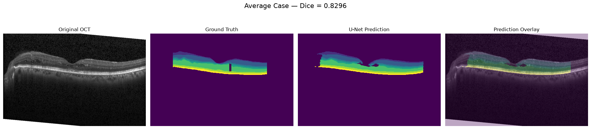
A representative (near-average) case: segmentation tracks the boundaries closely across most layers.

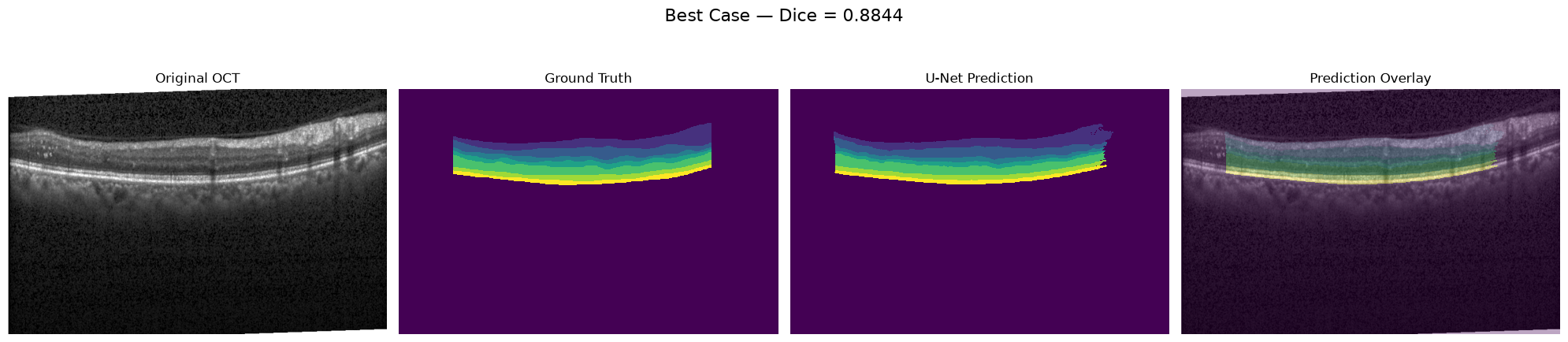
The best validation case: boundaries are nearly indistinguishable from the manual annotation.

The worst validation case, and the most informative one: errors cluster around the same thin middle layers (3 and 4) that scored lowest on Dice, rather than being scattered randomly across the scan.

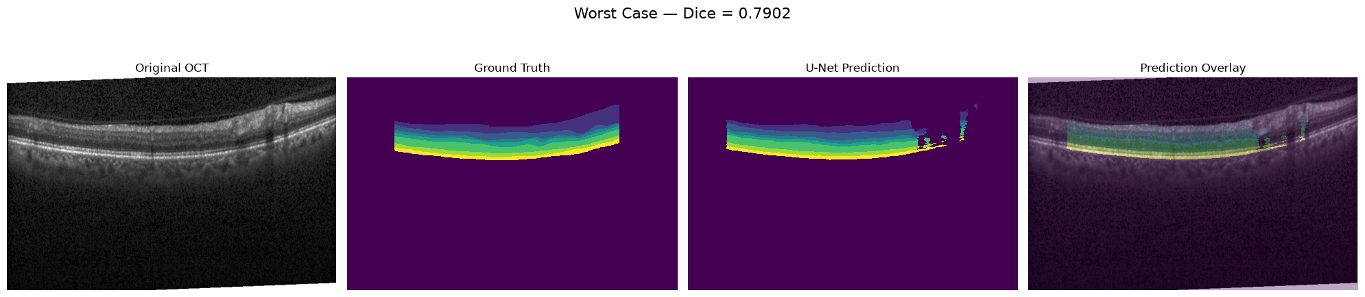
That consistency (errors concentrating in the same anatomically harder layers rather than appearing randomly) is a better sign than the aggregate Dice score alone. It suggests the model is struggling with genuinely ambiguous boundaries, not failing arbitrarily.

Limitations

This is a proof-of-concept, not a clinical tool. The annotated set is small (110 B-scans, 10 subjects), evaluation is on a held-out subset of the same dataset rather than an external cohort, segmentation is 2D per B-scan rather than volumetric, and there’s no formal analysis of how much the two human graders disagreed with each other in the first place. That matters, because a model can’t be meaningfully more “correct” than its ground truth.

Why this project matters to me

The result I care about most isn’t the Dice score. It’s having built, myself, a full path from raw ophthalmic imaging data to a validated quantitative pipeline: data interpretation → image processing → anatomical representation → machine learning → quantitative evaluation. That’s the actual skill I was trying to build.

It’s also pointed me toward what I want to work on next. Retinal layer segmentation in 2D is a reasonable starting point, but the clinically interesting question is volumetric: how do you go from individual B-scan segmentations to a reconstructed 3D surface, correct for scan geometry and de-warping, and extract meaningful curvature or shape metrics about the posterior eye? That’s the direction I’m heading, combining the segmentation and image-processing groundwork from this project with geometric analysis to build quantitative approaches to vision science that start from my clinical background rather than in spite of it.